Description
Understanding options is one thing — getting clean, reliable options data is another. If you want to analyze your strategies, validate pricing, or simply explore whether a vertical spread makes sense, you first need access to the option chain. Different online tools allow you to get the option data programmatically, and even using the API of some brokers can be useful. I am going to use here yfinance, which works pretty well with Python.
Why Fetching Option Chains Matters
An option chain is essentially the entire menu of available options for a given underlying — strikes, expirations, bid/ask prices, implied volatilities, and more. You need option chain data when you want to:
- Evaluate multi-leg options strategies: Spreads, iron condors, calendars — all require knowing which strikes and expirations are available, and at what prices.
- Compare premiums across different expirations: Understanding term structure helps you select the expiration that best aligns with your edge or time horizon.
- Compute theoretical vs. market pricing: If you’re building models (like for your seasonality-based SPY strategy), you need accurate mid-prices for each leg.
Without programmatic access to option chains, automation is nearly impossible. Indeed, to trade the seasonal pattern, similar to the one I have described in the previous blog, for the SPY seasonal window from October 26 to December 7, we can play around with different strikes and expiration dates to find the best trade and to identify a risk/reward ratio more suitable for our trading profile. Furthermore, with a bull call spread or bull put spread possibilities, we can make a better comparison before we send the trade to the broker.
Fetching SPY’s Option Chain With Yfinance
Below is a simple, readable Python script to get the available expirations and pull the option chain for one of them.
import yfinance as yf

ticker = yf.Ticker("SPY")

# List all available option expiration dates
expirations = ticker.options
print("Available expirations:")
print(expirations)

# Choose an expiration (e.g., the one closest to December 7)
expiration = expirations[0]  # replace with the one you want
print("\nUsing expiration:", expiration)

# Fetch the option chain for this date
opt_chain = ticker.option_chain(expiration)

calls = opt_chain.calls
puts = opt_chain.puts

print("\nCALLS:")
print(calls.head())

print("\nPUTS:")
print(puts.head())As of the time of writing, the following expirations are available:
(‘2025-11-24’, ‘2025-11-25’, ‘2025-11-26’, ‘2025-11-28’, ‘2025-12-01’, ‘2025-12-02’, ‘2025-12-03’, ‘2025-12-04’, ‘2025-12-05’, ‘2025-12-12’, ‘2025-12-19’, ‘2025-12-26’, ‘2025-12-31’, ‘2026-01-02’, ‘2026-01-16’, ‘2026-01-30’, ‘2026-02-20’, ‘2026-02-27’, ‘2026-03-20’, ‘2026-03-31’, ‘2026-04-30’, ‘2026-06-18’, ‘2026-06-30’, ‘2026-09-18’, ‘2026-09-30’, ‘2026-12-18’, ‘2027-01-15’, ‘2027-03-19’, ‘2027-06-17’, ‘2027-12-17’, ‘2028-01-21’)
I am going to use the expiration 2025-12-12, since it is the first that comes after the date of the end of the seasonal window.
Building the SPY Vertical Spread
Let’s say the seasonality analysis suggests that SPY tends to rise ~3–5% during the Oct–Dec window. Assume SPY is trading at $660. A 5% seasonal move suggests an upside target of roughly $686.
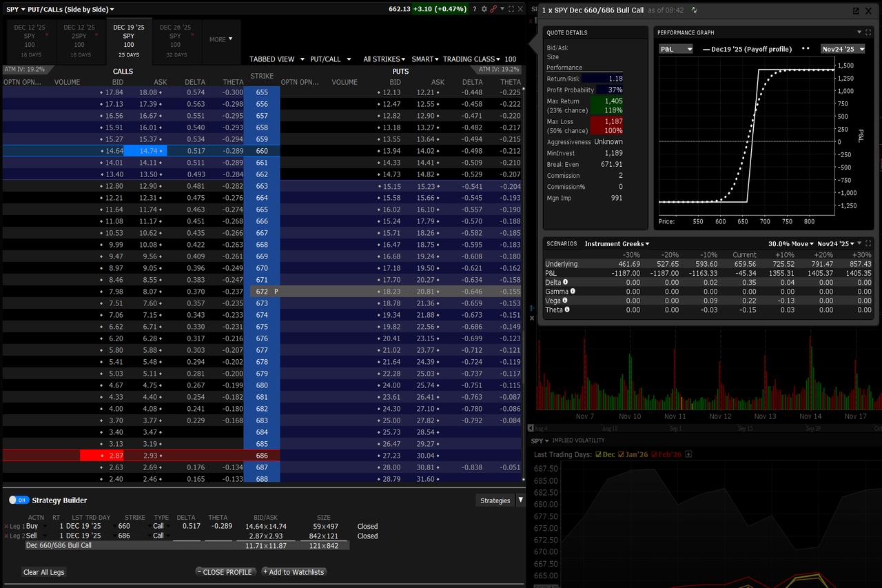
So you might build a bull call spread like this:
- Buy 660 call
- Sell 686 call
- Choose an expiration shortly after December 7
Let’s fetch the data for the specific case
ticker = yf.Ticker("SPY")
expiration = "2025-12-12"  # example

chain = ticker.option_chain(expiration)
calls = chain.calls

K1 = 660
K2 = 686

# Select legs
long_call  = calls[calls['strike'] == K1].iloc[0]
short_call = calls[calls['strike'] == K2].iloc[0]

# Compute mid prices
long_mid  = (long_call['bid'] + long_call['ask']) / 2
short_mid = (short_call['bid'] + short_call['ask']) / 2

debit = long_mid - short_mid
max_profit = K2 - K1 - debit  # (525 - 500 = 25 spread width)

# Compute breakeven
breakeven = K1 + debit

print("Long call mid price:", long_mid)
print("Short call mid price:", short_mid)
print("Net debit:", debit)
print("Breakeven price:", breakeven)
print("Max profit:", max_profit)This gives you:
- Cost for entering the spread: 11.06$
- Maximum profit: 14.93$
- Breakeven price: 671.07$
- Risk/Reward ratio: 0.74
If you try to run the script, you are going to find different numbers, but the concepts remain identical.
With the option chain fetched automatically, you can build your spreads dynamically and scan multiple expiration dates. The strike selection can also be optimized to have a different risk/reward ratio.
This is the bridge between quantitative idea → tradable strategy.
Visualize the Payoff
Add this piece of code to visualize the payoff:
import numpy as np
import matplotlib.pyplot as plt

def bull_call_spread_payoff(S, K1, K2, debit):
    return np.maximum(0, S - K1) - np.maximum(0, S - K2) - debit


S = np.linspace(620, 710, 300)
payoff = bull_call_spread_payoff(S, K1, K2, debit)

plt.figure(figsize=(10,6))
plt.plot(S, payoff, label='Bull Call Spread Payoff')
# Background colors
plt.axhspan(0, max(payoff), alpha=0.15)
plt.axhspan(min(payoff), 0, alpha=0.15, color='red')

plt.axvline(breakeven, color='green', linestyle='--', linewidth=1.5, label=f'Breakeven ({breakeven:.2f})')


plt.axhline(0, color='black', linewidth=1)
plt.title("Bull Call Spread – Payoff at Expiration")
plt.xlabel("SPY Price at Expiration")
plt.ylabel("Profit / Loss")
plt.grid(True)
plt.legend()
plt.show()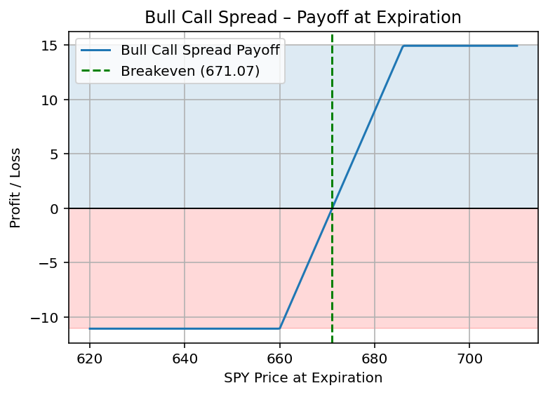
To make the payoff chart more intuitive, I added a dashed green line to mark the breakeven point, calculated as: Breakeven = K + debit. So if I buy the 660$ call and pay a net debit of 11$, the breakeven price is 671$.
Above this price, the position enters profit territory; below it, the loss is capped at the upfront debit.
The breakeven line makes it much easier to evaluate whether the spread’s structure matches your directional thesis—and whether the seasonal move you’re targeting has historically been sufficient to reach profitability.
Final Thoughts
Fetching option chain data is the first building block in turning market insights into actual trades. Whether you’re analyzing seasonal edges, volatility patterns, or simple directional setups, having programmatic access to the data opens the door to automation and more informed decision-making.
If you want the next article sent directly to your inbox, make sure you’re subscribed to the newsletter.
This is the mindset behind The Quantitative Edge — simple ideas, implemented cleanly, that scale into powerful tools for data-driven trading.
Statemi bene!