Description
Every time I place a bull put spread or sell a cash-secured put, I’m relying, often implicitly, on a fundamental relationship between the price of a call and the price of a put. It’s called Put-Call Parity, and it is, without exaggeration, the gravitational constant of the options market.
Most retail traders have never heard of it. And yet, it runs silently beneath every options chain, every spread, every synthetic position. Market makers check it millions of times per second.
In this post, I want to break it down the way a physicist would: start with the intuition, prove it with logic, and then build a Python tool you can run yourself to spot when the market drifts out of balance.
Before the Equation: European vs. American Options
Before we can talk about Put-Call Parity, we need to settle one mechanical point: when can you actually exercise an option? This is called the exercise style, and it comes in two flavors:
- European style: you can only exercise at expiration. Not before, not after.
- American style: you can exercise at any point before expiration.
What about a classical physics analogy I usually like to share?
The European style option can be considered as a quantum measurement. In quantum mechanics, a particle is described as a wave; it carries energy, it moves, it exists, but you can only measure the physical properties once, in a predetermined moment, because it loses the information and the wave function collapses at this precise instant. Before that instant, the system is alive but untouchable. A European option works the same way: the right to exercise exists, it has value, but you can only act on it at a single point in time. SPX options work this way.
The American style option is like a particle detector with a configurable trigger. You set the detector to fire the moment the signal crosses your threshold, and it will respond at any point within the measurement window, not just at the end. You don’t schedule the observation; you set the condition and wait. The moment the underlying hits your level, you can act. This is how almost all individual equity options (AAPL, TSLA, NVDA) and most ETF options work.
The names have nothing to do with geography. They define the timeline of your rights.
Why does this matter? Because an American option gives you everything a European option gives you, plus the flexibility to act early. That extra flexibility has a price: it’s called the Early Exercise Premium. American options are always worth at least as much as their European equivalents.
When Does Early Exercise Actually Make Sense?
Buying an American style option comes with a genuine advantage: the right to exercise at any point before expiration. But when is that right worth using?
Almost never! Here’s why.
When you exercise early, you instantly destroy whatever time value (Theta) remains in the option. If your position is profitable, selling the option in the market is almost always smarter, since you capture both the intrinsic value and the remaining time premium.
But there are two genuine exceptions:
- Deep In-the-Money Puts and the Time Value of Money:
Imagine you own a Put with a $100 strike, and the underlying is trading at $2, essentially worthless. You could wait 6 months until expiration to collect your $98. But why wait? If you exercise today, you get the $98 now and can immediately put it to work earning interest. In this case, the time value of money beats the remaining option time value. - Call Options Before a Large Dividend:
If a stock is about to pay a significant dividend tomorrow, you don’t collect it as an option holder; you collect it only as a stockholder. Exercising your call today, buying the shares, and capturing the dividend can make mathematical sense if the dividend exceeds the remaining time value in the option.
Outside these two cases, don’t exercise early. Sell the option instead.
Put-Call Parity: The Equation
Now we get to the core. Put-Call Parity applies strictly to European options, because the clean math requires that all payoffs happen at the same moment (expiration). The relationship is:
where:
- C = Price of the European Call
- P = Price of the European Put
- S = Current stock price (Spot)
- K = Current stock price (Spot)
- PV(K) = Present value of the strike price = K × e^(-rT)
Both sides of this equation must be equal. Always. Or arbitrage destroys the imbalance.
The Logical Proof (No Algebra Required)
Here’s the physicist’s approach: build two portfolios, hold them to expiration, and compare what’s in your hands.
Portfolio A — The “Fiduciary Call” (Left side of the equation):
- Buy one Call option (C)
- Deposit enough cash in a risk-free account so that it grows to exactly K at expiration → that’s PV(K) today
Portfolio B — The “Protective Put” (Right side of the equation):
- Buy one share of the stock (S)
- Buy one Put option as insurance (P)
Now fast-forward to expiration. Two scenarios:
Scenario 1: Stock finishes BELOW the strike (S_T < K)
- Portfolio A: The call expires worthless. The cash account matures to K. You hold K in cash.
- Portfolio B: The stock is down, but the put kicks in. You sell the stock at K via the put. You hold K in cash.
Same result.
Scenario 2: Stock finishes ABOVE the strike (S_T > K)
- Portfolio A: The call is deep in the money. You use the K cash from the bond to exercise the call and buy the stock. You hold one share of stock.
- Portfolio B: The put expires worthless. You already own the stock. You hold one share of stock.
Same result.
In every possible future state of the world, Portfolio A and Portfolio B deliver the identical payoff. Therefore, they must cost the same today. That is Put-Call Parity. It’s not a theory. It’s a logical inevitability.
What Happens When Parity Breaks?
Imagine Portfolio B (Put + Stock) is trading cheap, and Portfolio A (Call + Cash) is trading expensive.
A market maker instantly:
- Buys the cheap portfolio: buy the Put, buy the Stock
- Sells the expensive portfolio: sell the Call, borrow the Cash
Because both portfolios deliver the same payoff at expiration, the future cash flows cancel perfectly. The market maker pockets the price difference today as risk-free profit. Zero risk. Guaranteed gain.
The moment this trade executes at scale, the buying pressure pushes prices up on the cheap side, the selling pressure pushes prices down on the expensive side, and parity is restored. This happens in milliseconds.
Rearranging the Equation: Synthetic Positions
This is where it gets interesting for a systematic trader. Put-Call Parity lets you construct any leg synthetically:
# Rearranging for the Call:
C = P + S - PV(K)      → A Call = Put + Stock - Bond

# Rearranging for the Put:
P = C + PV(K) - S      → A Put = Call + Bond - Stock

# Rearranging for the Stock:
S = C - P + PV(K)      → Stock = Call - Put + Bond

# Rearranging for a Risk-Free Bond:
PV(K) = P + S - C      → Bond = Put + Stock - Call
This is how brokers build synthetic positions, how market makers hedge, and how you can think about your spreads in a completely different light.
Python: Checking Put-Call Parity in Real Time
Let’s make this concrete. Here’s a Python script that fetches real option data and checks whether parity holds — and flags the violation if it doesn’t.
We’ll use yfinance to pull live option chain data and check parity for a liquid equity like SPY (American style, so the check is approximate) or ideally SPX (European style, where it’s exact).
import yfinance as yf
import numpy as np
import pandas as pd
from datetime import datetime
def check_put_call_parity(ticker: str, expiry: str, risk_free_rate: float = 0.05):
"""
Checks Put-Call Parity violations for a given ticker and expiry.
Parameters:
ticker: Stock symbol (e.g., 'SPY')
expiry: Expiration date string (e.g., '2026-05-16')
risk_free_rate: Annual risk-free rate (default: 5%)
"""
stock = yf.Ticker(ticker)
S = stock.history(period="1d")["Close"].iloc[-1] # Current spot price
# Time to expiry in years
T = (datetime.strptime(expiry, "%Y-%m-%d") - datetime.now()).days / 365
# Pull option chain
chain = stock.option_chain(expiry)
calls = chain.calls[["strike", "lastPrice"]].rename(columns={"lastPrice": "call_price"})
puts = chain.puts[["strike", "lastPrice"]].rename(columns={"lastPrice": "put_price"})
# Merge on strike
merged = pd.merge(calls, puts, on="strike")
merged = merged[(merged["call_price"] > 0.10) & (merged["put_price"] > 0.10)] # filter thin strikes
# Put-Call Parity: C + PV(K) = P + S
merged["PV_K"] = merged["strike"] * np.exp(-risk_free_rate * T)
merged["lhs"] = merged["call_price"] + merged["PV_K"] # C + PV(K)
merged["rhs"] = merged["put_price"] + S # P + S
merged["deviation"] = merged["lhs"] - merged["rhs"]
print(f"\n{'='*60}")
print(f" Put-Call Parity Check | {ticker} | Expiry: {expiry}")
print(f" Spot Price (S) = ${S:.2f} | Risk-Free Rate = {risk_free_rate*100:.1f}%")
print(f"{'='*60}")
print(f"{'Strike':>10} {'Call':>8} {'Put':>8} {'LHS':>10} {'RHS':>10} {'Deviation':>12}")
print("-"*60)
for _, row in merged.iterrows():
flag = " ⚠️" if abs(row["deviation"]) > 0.5 else ""
print(f"{row['strike']:>10.1f} {row['call_price']:>8.2f} {row['put_price']:>8.2f} "
f"{row['lhs']:>10.2f} {row['rhs']:>10.2f} {row['deviation']:>+12.2f}{flag}")
print(f"\nMax deviation: ${merged['deviation'].abs().max():.2f}")
print(f"Mean deviation: ${merged['deviation'].abs().mean():.2f}")
return merged
# --- Run it ---
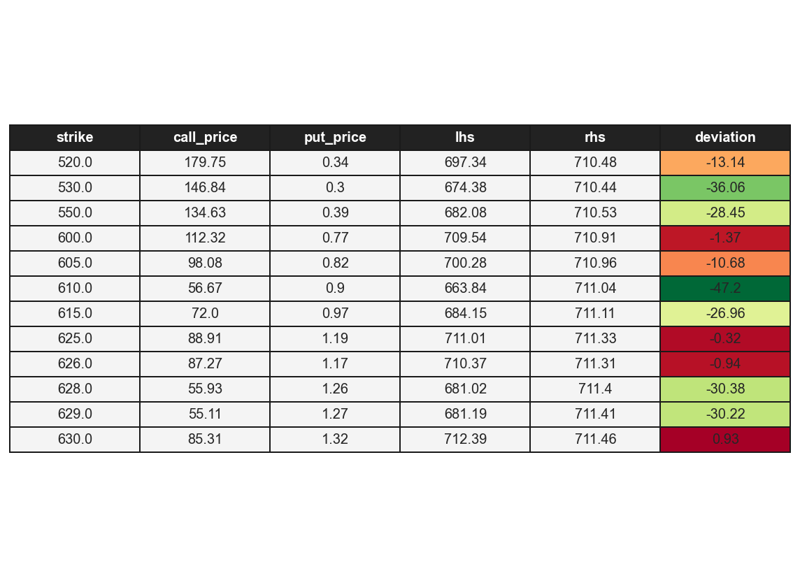
df = check_put_call_parity("SPY", "2026-05-22", risk_free_rate=0.053)
On liquid strikes near the money, you’ll find that parity holds within a few cents; the bid-ask spread is often the entire “violation.” That’s the market working exactly as it should.
On deep out-of-the-money or thinly traded strikes, you’ll see larger deviations. These aren’t free money; they reflect illiquidity, transaction costs, and the bid-ask spread. True arbitrage requires you to execute both legs simultaneously at the market price, which requires scale.
But the exercise is illuminating. It shows you that the options market is internally consistent. The prices you see are not random numbers; they’re bound together by a mathematical equilibrium enforced by armies of market makers running exactly this check.
A Practical Example by Hand
Let’s run the numbers manually, assuming a 0% risk-free rate for simplicity (so PV(K) = K):
| Variable | Value |
|---|---|
| Spot price (S) | $195.00 |
| Strike (K) | $195.00 |
| Call price (C) | $4.20 |
| Put price (P) | $2.10 |
Check:
- Left side: C + K = $4.20 + $195.00 = $199.20
- Right side: P + S = $2.10 + $195.00 = $197.10
Deviation = +$2.10
The call is overpriced (or the put is underpriced) by $2.10. If you could execute this at scale with no transaction costs:
- Buy the cheap portfolio (buy the put, buy the stock): pay $197.10
- Sell the expensive portfolio (sell the call, invest K in cash): receive $199.20
- Pocket $2.10 per share, risk-free, regardless of where the stock ends up
In reality, bid-ask spreads and slippage eat into this. But this is the exact logic that market makers run.
Final Thoughts
Put-Call Parity is one of those concepts that looks theoretical until you realize it’s actively enforced by every serious market participant in real time.
For a systematic options trader, the key takeaways are practical:
You can construct any position synthetically. A long call is equivalent to a long put + long stock + short bond. This matters when you’re thinking about the risk profile of your spreads.
Violations signal something. If you see an apparent parity breakdown, before assuming you found free money, check the bid-ask spread, the dividend schedule, and whether the options are American style (early exercise premium distorts the clean formula).
European vs. American matters. The parity formula is exact for European options (SPX). For American options (SPY, individual equities), it becomes an inequality; the American price is always ≥ the European equivalent due to the early exercise premium.
The market is not random. It is constrained. The more of these constraints you understand, the better your edge.
This is the mindset behind The Quantitative Edge — simple ideas, implemented cleanly, that scale into powerful tools for data-driven trading.
Statemi bene!
If you found this useful, you might also enjoy: