Description
Implied volatility tells you how expensive options are. But expensive compared to what? IV Rank answers that question. In this post, we break down IV Rank and IV Percentile: what they measure, how to calculate them, and how to use them in Python to decide when conditions are truly favorable for selling premium.
Introduction
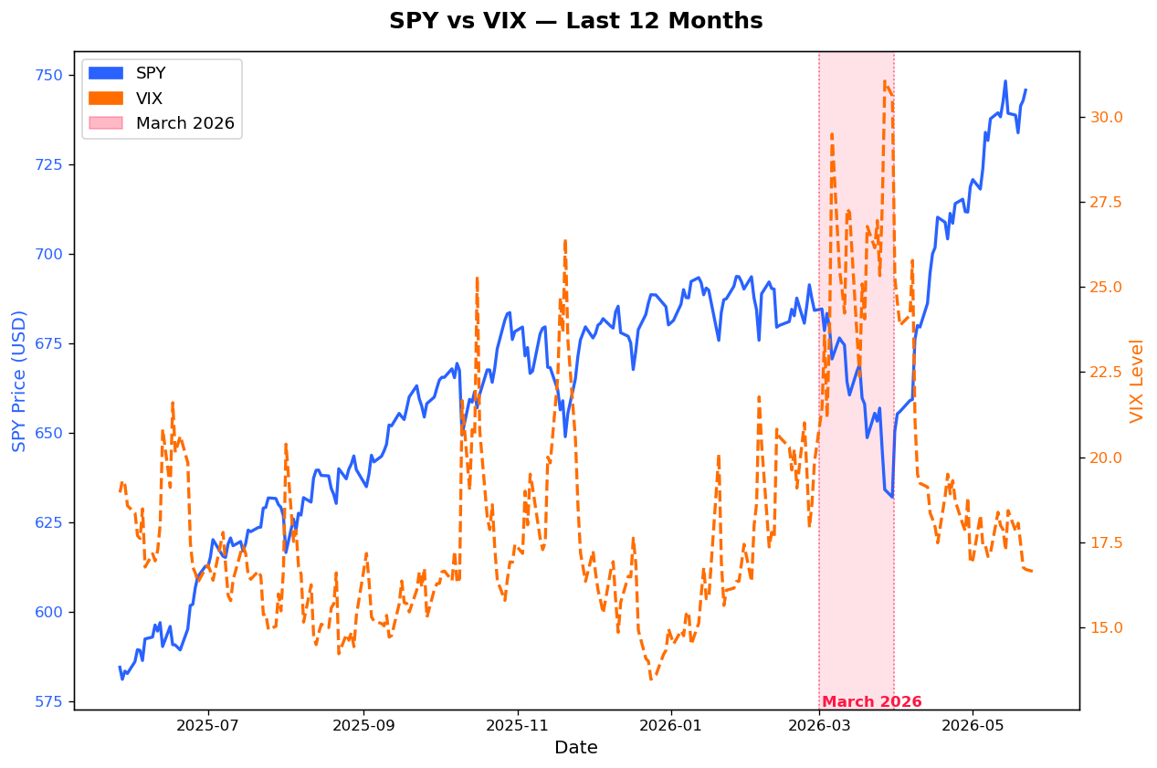
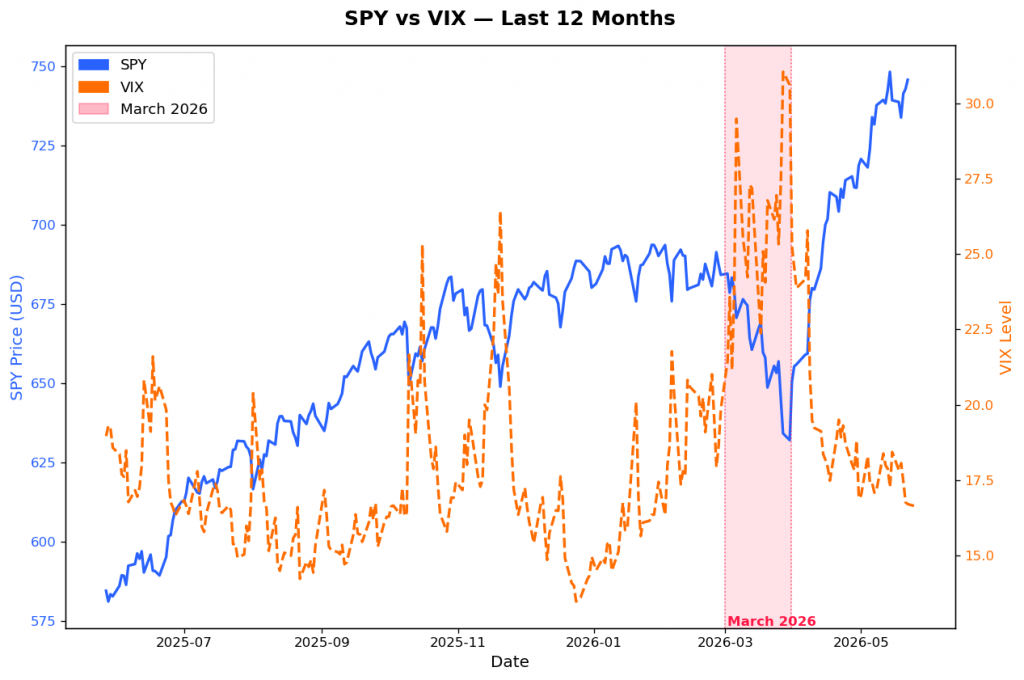
March 2026. The VIX spikes above 25. The S&P 500 drops over 4% in a single month. Your inbox fills with messages: “IV is elevated: great time to sell options!”
But is it really?
A VIX at 25 is high compared to January. But what if this ticker you’re watching normally trades with implied volatility around 60%? Suddenly, 25% IV isn’t rich at all; it’s actually cheap. Selling premium there is the wrong trade.
This is the core problem. Raw implied volatility gives you a number. It does not tell you whether that number is high, low, or somewhere in between for that specific instrument. Without context, you’re flying blind.
IV Rank fixes that. It is a single number, between 0 and 100, that tells you exactly where the current IV sits relative to its own recent history. It transforms an absolute number into a relative signal, and for premium sellers, that distinction is everything.
The Problem with Raw Implied Volatility
Let’s say you’re looking at two tickers:
- Ticker A has an implied volatility of 35%
- Ticker B has an implied volatility of 35%
Same number. Same trade? Not even close.
If Ticker A normally trades between 20% and 40% IV over the past year, then 35% is near the top of its range. So this can be a great moment to sell premium.
If Ticker B normally trades between 30% and 80% IV, then 35% is near the bottom. So the premium is cheap, and selling here puts you at a disadvantage.
Same IV. Completely different context. That’s why raw IV alone is a misleading signal. You need to normalize it.
IV Rank: The Formula
IV Rank normalizes current implied volatility against the 52-week high and low of IV for that specific instrument. The formula is clean:
IV Rank = (Current IV – 52-week IV Low) / (52-week IV High – 52-week IV Low) × 100
The result is a number between 0 and 100:
- IVR = 0 means the current IV is at the lowest point of the past year
- IVR = 100 means the current IV is at the highest point of the past year
- IVR = 50 means the current IV sits exactly in the middle of its annual range
Simple numerical example:
- 52-week IV Low: 18%
- 52-week IV High: 55%
- Current IV: 42%
- IVR = (42 – 18) / (55 – 18) × 100 = 24 / 37 × 100 ≈ 64.9
IVR of ~65. IV is relatively elevated. Conditions favor premium selling.
IV Rank vs IV Percentile: What’s the Difference?
These two metrics are often confused. They measure different things.
IV Rank asks: Where does current IV sit within its 52-week range? It uses only the high and the low, nothing in between.
IV Percentile asks: What percentage of the past year did IV close below the current level? It looks at every single daily closing IV value.
Here’s a simple table to make the difference concrete:
| Metric | What it measures | Sensitive to outliers? |
|---|---|---|
| IV Rank | Position between 52W high and low | Yes — one extreme spike distorts the range |
| IV Percentile | % of days IV was lower than today | No — outliers are just one data point |
Example: Suppose a stock had one massive volatility spike six months ago (earnings miss, stock dropped 30%). That spike pushed the 52-week IV high to 90%. Now IV is at 45%.
- IV Rank: (45 – 18) / (90 – 18) × 100 = 37.5 → looks low
- IV Percentile: 45% was higher than 80% of all daily closes → actually quite elevated
In this case, IV Percentile gives a more accurate picture because it is not distorted by that single spike.
Which one to use?
Both. They complement each other. IV Rank gives you a quick read on range position. IV Percentile gives you a distribution-based view. When both are elevated, you have a strong confluence signal. When they diverge, dig deeper before entering.
Python Implementation
If you are an Interactive Brokers user, you have access to something better than a proxy: real implied volatility data, pulled directly from IBKR’s options pricing engine via the TWS API.
The library we use is ib_insync — the cleanest Python wrapper for the TWS API. Install it with: pip install ib_insync. You also need TWS or IB Gateway running locally, with API access enabled (Edit → Global Configuration → API → Enable ActiveX and Socket Clients).
from ib_insync import IB, Stock
import pandas as pd

def fetch_iv_from_ibkr(ticker: str, ib: IB) -> pd.Series:
    """
    Fetch 1-year of daily implied volatility from IBKR TWS API.
    Returns a Series of IV values (as decimals, e.g. 0.35 = 35%).
    """
    contract = Stock(ticker, 'SMART', 'USD')
    ib.qualifyContracts(contract)

    bars = ib.reqHistoricalData(
        contract,
        endDateTime='',
        durationStr='1 Y',
        barSizeSetting='1 day',
        whatToShow='OPTION_IMPLIED_VOLATILITY',  # real IV, not HV proxy
        useRTH=True,
        formatDate=1
    )

    if not bars:
        raise ValueError(f"No IV data returned for {ticker}")

    iv_series = pd.Series(
        [bar.close for bar in bars],
        index=[bar.date for bar in bars]
    ) * 100  # convert to percentage

    return iv_series.dropna()
The key is whatToShow='OPTION_IMPLIED_VOLATILITY'. This is IBKR’s own IV calculation derived from the live options chain — the real thing, not a historical volatility approximation.
Step 2: Compute IV Rank and IV Percentile
The math is identical to before. The only thing that changed is the data source.
def iv_rank(iv: pd.Series) -> float:
    """
    IV Rank: where is current IV within its 52-week range?
    Returns a value between 0 and 100.
    """
    current = iv.iloc[-1]
    iv_low  = iv.min()
    iv_high = iv.max()

    if iv_high == iv_low:
        return 50.0

    return round((current - iv_low) / (iv_high - iv_low) * 100, 1)


def iv_percentile(iv: pd.Series) -> float:
    """
    IV Percentile: % of days IV closed below current level.
    Returns a value between 0 and 100.
    """
    current = iv.iloc[-1]
return round((iv < current).sum() / len(iv) * 100, 1)Step 3: The full screener
def ivr_screener_ibkr(tickers: list) -> pd.DataFrame:
    """
    Screen a watchlist for IV Rank and IV Percentile using IBKR real IV data.
    Requires TWS or IB Gateway running locally.
    """
    ib = IB()
    ib.connect('127.0.0.1', 7497, clientId=1)  # use 7496 for live, 7497 for paper

    results = []

    for ticker in tickers:
        try:
            iv = fetch_iv_from_ibkr(ticker, ib)
            current_iv = round(iv.iloc[-1], 1)
            ivr        = iv_rank(iv)
            ivp        = iv_percentile(iv)

            results.append({
                "Ticker":        ticker,
                "Current IV%":   current_iv,
                "IV Rank":       ivr,
                "IV Percentile": ivp,
                "Signal":        "✅ Sell Premium" if ivr >= 50 and ivp >= 50 else "⏳ Wait",
            })

        except Exception as e:
            print(f"⚠️ Skipping {ticker}: {e}")

    ib.disconnect()

    df = pd.DataFrame(results)
    df = df.sort_values("IV Rank", ascending=False)
    return df


# --- Run the screener ---
watchlist = ["AAPL", "MSFT", "NVDA", "KO", "AMZN", "GLD", "SPY", "QQQ", "MCD", "HAS"]

df = ivr_screener_ibkr(watchlist)
print(df.to_string(index=False))Sample Output (25/05/2026):
============================================================
  RESULTS
============================================================
Ticker  Current IV%  52W IV Low%  52W IV High%  IV Rank  IV Percentile       Signal
   MCD         19.5         14.2          24.3     52.1           56.6 Sell Premium
  MSFT         26.8         15.9          40.1     44.9           57.8         Wait
   QQQ         20.4         14.4          29.2     40.4           70.5         Wait
   HAS         31.4         23.2          45.6     36.8           57.0         Wait
    KO         16.8         12.8          23.6     36.6           39.4         Wait
  AAPL         21.3         16.8          33.3     27.5           10.8         Wait
   GLD         20.7         13.6          42.8     24.2           47.0         Wait
  NVDA         36.7         31.2          54.2     23.9           38.6         Wait
   SPY         13.9         10.5          26.3     21.6           49.4         Wait
  AMZN         28.0         22.6          50.0     19.7           29.9         Wait
Two signals stand out immediately: MCD has both IVR and IVP well above 50. There is also an additional point. When volatility rank and seasonal edge align on the same ticker, that is a strong confluence. Two independent signals pointing in the same direction. And now, with real IV data from IBKR instead of a proxy, the signal is cleaner.
How to Use IV Rank in Premium Selling
IV Rank is a filter. It tells you when conditions are favorable — not which trade to take.
Here is how to think about it in the context of cash-secured puts and credit spreads:
When IVR is high (above ~50): Premium is expensive relative to recent history. You are being well-compensated for the risk you are taking. This is when selling makes sense: whether that is a cash-secured put, a bull put spread, or an iron condor. Time decay works in your favor, and if volatility contracts after your entry, the position gains value even faster.
When IVR is low (below ~30): Premium is cheap. You are not being compensated adequately for the risk. This is the environment where premium sellers get punished since you collect a thin credit, and any adverse move wipes it out with no cushion. This is the time to wait, not to force trades.
The confluence approach: Do not use IVR in isolation. Stack it with other filters:
- Quality stock or ETF you are comfortable owning (or holding through a drawdown)
- Neutral to bullish directional outlook (look for clear signals)
- IVR elevated — confirmed by IVP pointing in the same direction
- Seasonal edge, if available — timing your entry when the historical pattern also supports the trade
When all filters align, you have a high-conviction setup. When only one or two do, you wait. Discipline here is the most important edge.
A note on credit spreads: Bull put spreads benefit from IV Rank in a specific way. When IVR is high, you collect more premiums for the same spread width. Your break-even is further from the current price, and your probability of profit is higher. The same spread that generates $0.80 credit at IVR 20 might generate $1.80 at IVR 70. That is not a small difference — it completely changes the risk/reward of the position.
Final Thoughts
IV Rank is one of the simplest tools in the systematic trader’s toolkit. But simple does not mean unimportant: it means it works.
It answers the one question raw implied volatility can never answer on its own: Is this IV actually high?
The formula takes 30 seconds to understand. The Python implementation runs in under a minute. And the discipline to wait for high IVR before selling premium. This is what separates systematic traders from everyone else.
Use IV Rank as your entry gate. Use IV Percentile to validate. Stack them with your directional view, your quality filters, and your seasonal signals when available. Then act with conviction.
The data tells you when to trade. Your job is to listen.
This is the mindset behind The Quantitative Edge — simple ideas, implemented cleanly, that scale into powerful tools for data-driven trading.
Statemi bene!
If you found this useful, you might also enjoy: