Description
When you’re running a backtest, every line of code depends on a silent assumption:
The data actually reflects what happened in the market.
But that assumption can break down — not because of your model, but because of something much smaller and easier to overlook: price adjustments.
Whether your price series is adjusted or unadjusted can completely change your results, sometimes flipping a losing strategy into what looks like a winner.
Let’s unpack why.
(For a detailed analysis of the main differences between adjusted and unadjusted prices: Read More)
How Adjustments Are Calculated
Adjustments are applied retroactively by multiplying past prices by a cumulative adjustment factor derived from corporate events. This factor ensures that the total return is preserved through time.
If a company pays a dividend or splits shares, the historical prices before that event are scaled so that the price series remains continuous.
import yfinance as yf
import matplotlib.pyplot as plt

# Download historical data for Altria
aapl = yf.Ticker("AAPL")
data = aapl.history(period='5y',interval='1d', auto_adjust=False)

# Compute the adjustment factor
data['Adjustment Factor'] = data['Adj Close'] / data['Close']

# Compute the "manually adjusted" price for verification
data['Manual Adj Close'] = data['Close'] * data['Adjustment Factor']It demonstrates the logic behind adjustment for splits and dividends, and computes the adjustment factor that transforms the unadjusted “Close” into the “Adjusted Close.”
When Adjusted Prices Can Mislead You
Despite their advantages, adjusted prices can also be misleading — if you use them in the wrong context.
- Execution-level simulation: Adjusted prices never actually traded. You can’t “buy” a share at a split-adjusted price from five years ago.
- Corporate action research: If you’re studying the effect of dividends or splits, adjustment hides those effects.
- Backtesting intraday or high-frequency strategies: Intraday data usually doesn’t include adjustments — applying them incorrectly can distort your results.
A Backtest Example
Let’s see how the choice of price data affects a simple backtest. We’ll use a moving average crossover strategy — one of the simplest momentum systems — and run it twice:
- Using unadjusted prices (raw closing prices)
- Using adjusted prices (total-return data)
import yfinance as yf
import pandas as pd
import matplotlib.pyplot as plt

msft = yf.Ticker("MSFT")
data = msft.history(period='10y',interval='1d', auto_adjust=False)

# Create two datasets: one adjusted, one unadjusted
unadj = data.copy()
adj = data.copy()
adj["Close"] = adj["Adj Close"]

# Simple moving average crossover strategy
def sma_strategy(df, short=50, long=200):
    df = df.copy()
    df["SMA_short"] = df["Close"].rolling(short).mean()
    df["SMA_long"]= df["Close"].rolling(long).mean()
    df["Signal"] = (df["SMA_short"] > df["SMA_long"]).astype(int)
    df["Return"] = df["Close"].pct_change()
    df["Strategy"] = df["Signal"].shift(1) * df["Return"]
    df["Equity"] = (1 + df["Strategy"]).cumprod()
    return df

backtest_unadj = sma_strategy(unadj)
backtest_adj = sma_strategy(adj)

# Compare performance
plt.figure(figsize=(10,5))
plt.plot(backtest_unadj["Equity"], label="Unadjusted Prices", alpha=0.7)
plt.plot(backtest_adj["Equity"], label="Adjusted Prices", alpha=0.9)
plt.title(f"MSFT SMA Crossover Strategy — Adjusted vs. Unadjusted Data")
plt.legend()
plt.show()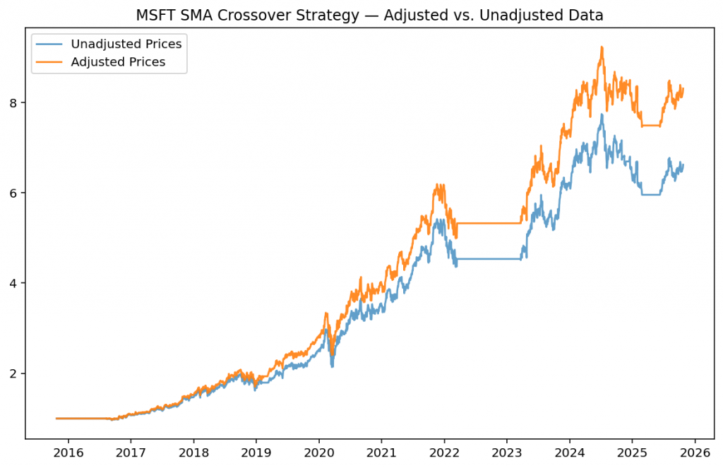
When you run this code, you’ll likely see different cumulative returns between the two datasets — sometimes noticeably so for dividend-paying stocks.
The adjusted-price backtest accounts for dividends and splits, representing total shareholder return. The unadjusted-price backtest ignores those distributions — it’s missing a key component of real performance.
In other words:
If you use unadjusted prices in a strategy that measures long-term performance, you’re not comparing apples to apples — you’re ignoring part of the fruit. 🍏
Practical Guidelines for Backtesting
Here’s a simple checklist for using price data correctly in backtesting:
✅ Use adjusted close for return calculations and signal generation.
✅ Use unadjusted open, high, low, and close for realistic order simulation (entry/exit prices).
✅ Always verify how your data provider defines “adjusted” — methods vary.
✅ Keep track of corporate actions separately if your strategy depends on them.
✅ Document your data assumptions — reproducibility matters.
A solid backtest isn’t just about models or indicators; it’s about data integrity.
Garbage in, garbage out — but sometimes, “garbage” means simply the wrong kind of price.
Final Thoughts
In physics, precision depends on calibration.
In trading, it depends on data consistency.
Backtests are only as honest as the data behind them — and adjusted prices are your calibration step, aligning historical signals with true economic reality.
This single detail often separates a robust quantitative system from one that only looks good on paper.
This is the mindset behind The Quantitative Edge — simple ideas, implemented cleanly, that scale into powerful tools for data-driven trading.
Statemi bene!