Description

In quantitative trading, like in physics, every model starts with data — and often, that means historical prices.
But not all price data is created equal.

One of the most overlooked — and misunderstood — aspects of market data is the distinction between adjusted and unadjusted stock prices.

It might seem like a small technical detail, but it’s often the difference between a strategy that looks profitable — and one that truly is making money. In this post, I’ll unpack why that distinction matters.

What Are Adjusted and Unadjusted Prices?

Let’s define them precisely.

• Unadjusted prices are the raw historical prices — exactly what was recorded on the trading day. They don’t account for stock splits, dividends, or corporate actions. These are the prices that investors actually saw and traded at.
• Adjusted prices, on the other hand, are mathematically modified to reflect those corporate events. The goal is to make historical prices comparable over time — as if the stock’s price history were continuous and unaffected by splits or dividends.

For example, if a company performs a 2-for-1 stock split, the share price halves while the number of shares doubles. If we don’t adjust for that, our chart will suddenly show the price dropping by 50% — even though nothing of real economic value changed.

Why Adjustments Matter

Corporate events can distort price history:

• Stock splits change the nominal price but not the company’s market capitalization.
• Dividends reduce the stock price temporarily when paid but represent real returns to shareholders.
• Mergers or spin-offs can change the structure of the underlying asset.

Without adjusting for these, you can introduce false signals into your backtests.
A simple moving average crossover might trigger prematurely.
A breakout system might interpret a split as a crash.

Let’s give an example for the Company Altria Group, ticker symbol MO:

import yfinance as yf
import matplotlib.pyplot as plt

# Download historical data for Altria
altria = yf.Ticker("MO")
data = altria.history(period='5y',interval='1d', auto_adjust=False)

# Compare adjusted vs. unadjusted close prices
plt.figure(figsize=(10,5))
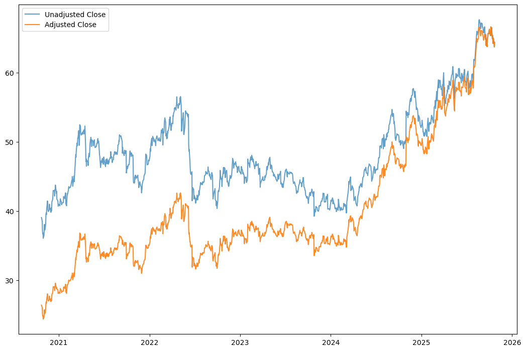
plt.plot(data['Close'], label='Unadjusted Close', alpha=0.7)
plt.plot(data['Adj Close'], label='Adjusted Close', alpha=0.9)
plt.title("MO — Adjusted vs. Unadjusted Close Prices")
plt.legend()
plt.show()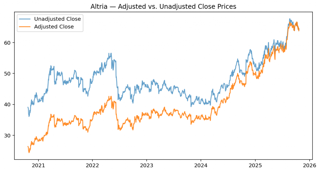

import yfinance as yf
import matplotlib.pyplot as plt

# Download historical data for Altria
altria = yf.Ticker("MO")
data = altria.history(period='5y',interval='1d', auto_adjust=False)

# Compare adjusted vs. unadjusted close prices
plt.figure(figsize=(10,5))
plt.plot(data['Close'], label='Unadjusted Close', alpha=0.7)
plt.plot(data['Adj Close'], label='Adjusted Close', alpha=0.9)
plt.title("MO — Adjusted vs. Unadjusted Close Prices")
plt.legend()
plt.show()

You’ll notice that the adjusted series is always lower over time — this accounts for dividends and splits.
It represents the total return version of the stock, suitable for backtesting.

Now, let’s compute returns for each and see how adjustments change the results.

import pandas as pd

returns_adj = data['Adj Close'].pct_change().dropna()
returns_unadj = data['Close'].pct_change().dropna()

comparison = pd.DataFrame({
    "Adjusted Return": returns_adj,
    "Unadjusted Return": returns_unadj 
})
comparison.describe()

import pandas as pd

returns_adj = data['Adj Close'].pct_change().dropna()
returns_unadj = data['Close'].pct_change().dropna()

comparison = pd.DataFrame({
    "Adjusted Return": returns_adj,
    "Unadjusted Return": returns_unadj 
})
comparison.describe()

The difference may seem small at first glance — 0.08% versus 0.05% — but it illustrates an important principle. Using adjusted prices, which account for dividends and splits, captures the true economic return of the stock. In contrast, the unadjusted return ignores these distributions, slightly underestimating performance.

When to Use Adjusted vs. Unadjusted Data

Here’s the key principle:

So, if your goal is to analyze performance or backtest a strategy, use adjusted prices. If you’re replicating execution, use unadjusted prices.

The adjusted price provides a smooth, continuous chart that allows for accurate long-term performance analysis, which is crucial for backtesting investment strategies and assessing historical returns. Be aware also that the current price is the unadjusted price, so it can be confusing to compare for immediate trading decisions. 

The Scientist’s Perspective: What You’re Actually Measuring

Think of adjusted data as normalized measurements.
Just as a physicist might calibrate an experiment to remove systematic bias, a trader adjusts prices to remove structural noise — the effects of corporate events that obscure true price movement.

When you use unadjusted prices in a backtest, you’re effectively comparing measurements taken under different conditions — before and after splits, dividends, and more.
That’s like comparing temperature readings from two sensors without first calibrating them.

Final Thoughts

In science, calibration ensures that measurements reflect reality. In trading, using adjusted data serves the same purpose — it aligns your analysis with the economic truth of a stock’s performance.

But like any calibration, it depends on context. When you’re simulating execution, you need the raw measurements. When you’re studying returns, you need the adjusted ones.

Knowing the difference — and when to use each — is one of the quiet but crucial skills that separates reliable backtests from illusions of profitability.

Because in quantitative trading, even the smallest assumption about data can become your biggest hidden bias.

In the next blog, I am going to give you a concrete example of how this often-overlooked tiny difference can give a distorted backtest result.

This is the mindset behind The Quantitative Edge — simple ideas, implemented cleanly, that scale into powerful tools for data-driven trading.

Statemi bene!