Description
When I first started backtesting strategies, I thought one long backtest was enough. It wasn’t. Markets change, conditions shift, and what worked in one year might fail in the next. That realization led me to walk-forward analysis — a systematic way to simulate how a strategy learns and adapts over time. In this post, I’ll show you how to generate the date sequences that make this method possible using Python.
Intro
In quantitative trading, walk-forward analysis helps you evaluate how a strategy performs over multiple, sequential time windows — instead of relying on a single backtest period.
It works by splitting your data into training and testing segments and then iteratively moving the window forward in time.
There are two common variants:
- Anchored Walk-Forward: The training period starts on the same date and expands over time.
- Unanchored Walk-Forward: Both training and testing periods “slide” forward, keeping a fixed window length.
This approach mimics how a live strategy evolves — learning from past data, applying what it learned to the next unseen period, and repeating.
Setting Up the Time Range
Let’s start by defining the start and end dates of your dataset. From there, we’ll create a small utility function that generates a continuous sequence of dates, returned as a pandas DatetimeIndex. This object is the foundation of our walk-forward framework, since it allows us to easily slice, shift, and segment time periods in a consistent way across all backtests.
import pandas as pd

def generate_date_range(start_date: str, end_date: str) -> pd.DatetimeIndex:
    """Generate a daily date range from start_date to end_date."""
    return pd.date_range(start=start_date, end=end_date, freq='D')

start_date = "2022-01-01"
end_date = "2025-05-31"
dates = generate_date_range(start_date, end_date)Generating the Walk-Forward Splits
Now we can write a simple function that loops through time and yields the appropriate training and testing date ranges.
from datetime import timedelta
from pandas.tseries.offsets import MonthEnd

def generate_walk_forward(dates: pd.DatetimeIndex, IS_months: int, OOS_months: int, anchored: bool = False):

    sequences = []
    start = dates.min()
    end = dates.max()

    if anchored:
        current_end = (start + pd.DateOffset(months=IS_months) - timedelta(days=1)) + MonthEnd(0)
        while True:
            IS_start = start
            IS_end = current_end
            OOS_start = IS_end + timedelta(days=1)
            OOS_end = (OOS_start + pd.DateOffset(months=OOS_months) - timedelta(days=1)) + MonthEnd(0)

            if OOS_end > end:
                break

            IS_dates = dates[(dates >= IS_start) & (dates <= IS_end)]
            OOS_dates = dates[(dates >= OOS_start) & (dates <= OOS_end)]

            sequences.append((IS_dates, OOS_dates))

            current_end = (current_end + pd.DateOffset(months=OOS_months)) + MonthEnd(0)

    else:

        current_start = start
        while True:
            IS_start = current_start
            IS_end = (IS_start + pd.DateOffset(months=IS_months) - timedelta(days=1)) + MonthEnd(0)
            OOS_start = IS_end + timedelta(days=1)
            OOS_end = (OOS_start + pd.DateOffset(months=OOS_months) - timedelta(days=1)) + MonthEnd(0)

            if OOS_end > end:
                break

            IS_dates = dates[(dates >= IS_start) & (dates <= IS_end)]
            OOS_dates = dates[(dates >= OOS_start) & (dates <= OOS_end)]

            sequences.append((IS_dates, OOS_dates))

            # Move forward by OOS length
            current_start = current_start + pd.DateOffset(months=OOS_months)

return sequencesThe core of our approach is the generate_walk_forward() function — a simple but flexible utility that automatically creates train/test time splits for walk-forward analysis. It takes a timeline of trading dates (as a pandas DatetimeIndex) and divides it into in-sample (IS) and out-of-sample (OOS) segments. The additional input information are IS_months, the number of months for the in-sample (training) period, and OOS_months, the number of months for the out-of-sample (testing) period.
Visualizing or Verifying the Splits
Before embedding this date split into your full backtest, it’s helpful to print or visualize your generated date ranges to make sure the logic matches your expectations.
import matplotlib.pyplot as plt
import matplotlib.dates as mdates
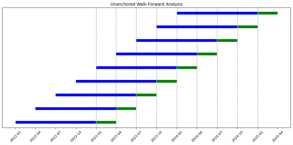
def plot_walk_forward_sequences(sequences, title="Walk-Forward Analysis"):
fig, ax = plt.subplots(figsize=(12, 6))
for i, (IS_dates, OOS_dates) in enumerate(sequences):
ax.plot(IS_dates, [i]*len(IS_dates), color='blue', linewidth=8, solid_capstyle='butt')
ax.plot(OOS_dates, [i]*len(OOS_dates), color='green', linewidth=8, solid_capstyle='butt')
if len(OOS_dates) > 0:
oos_start = OOS_dates.min()
ax.axvline(oos_start, color='gray', linestyle='--', linewidth=1)
ax.yaxis.set_visible(False)
ax.xaxis.set_major_locator(mdates.MonthLocator(interval=3))
ax.xaxis.set_major_formatter(mdates.DateFormatter('%Y-%m'))
plt.xticks(rotation=45)
plt.title(title)
plt.tight_layout()
plt.show()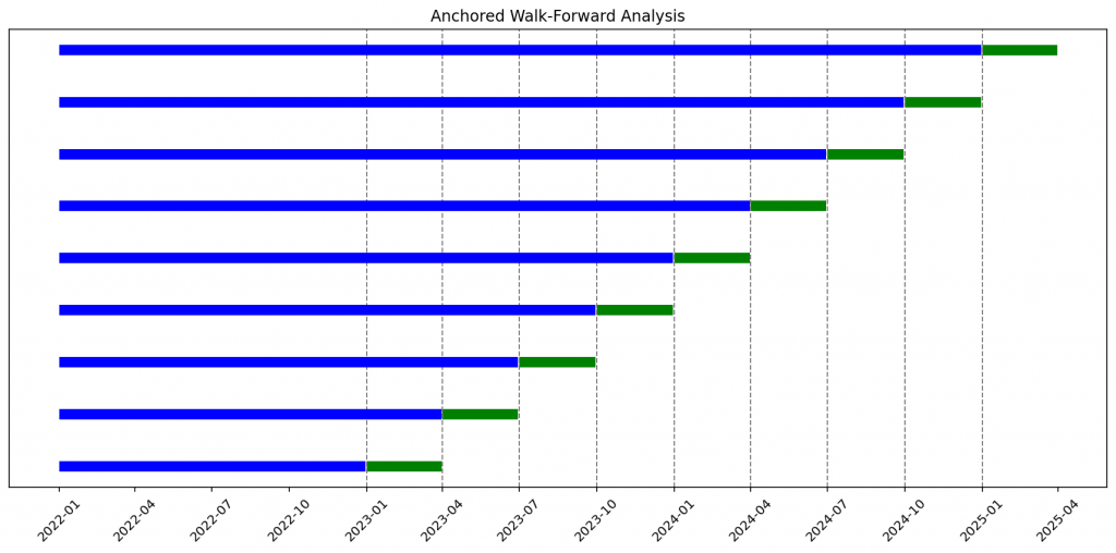
Example of usage of the provided code:
start_date = "2022-01-01"
end_date = "2025-05-31"
dates = generate_date_range(start_date, end_date)

# Walk-forward sequences
IS_months, OOS_months = 12, 3
unanchored_sequences = generate_walk_forward(dates, IS_months, OOS_months, anchored=False)
anchored_sequences = generate_walk_forward(dates, IS_months, OOS_months, anchored=True)
# Visualization
plot_walk_forward_sequences(unanchored_sequences, title="Unanchored Walk-Forward Analysis")
plot_walk_forward_sequences(anchored_sequences, title="Anchored Walk-Forward Analysis")Once verified, this utility becomes a drop-in component for your backtesting framework. Each generated range can dynamically feed into your model training and evaluation steps.
Final Thoughts
Walk-forward analysis forces your strategy to prove it can adapt over time, not just overfit to a single period.
By generating these date ranges programmatically, you can automate hundreds of rolling backtests — covering different time horizons, market conditions, and volatility regimes.
It’s a small utility with big implications for robust strategy design.
This is the mindset behind The Quantitative Edge — simple ideas, implemented cleanly, that scale into powerful tools for data-driven trading.
Statemi bene!