Description
Last month, I walked you through McDonald’s seasonal edge: 56 years of data, a 73% win rate, and a clear entry window from late March to early May. The theory was there. The data was there. But theory only gets you so far.
This time I want to show you something different. A real trade. Open to close. Numbers included.
The ticker is Hasbro (HAS). The instrument is a bull put spread. The result? Closed in 17 days with ~54% of the maximum profit captured, and a return on capital that no equity position could have matched with the same money.
Let me walk you through it.
The Tool Behind the Trade: SeasonHunter
Before I get into the trade itself, let me spend a minute on the tool that surfaced it, because without it, HAS wouldn’t have been on my radar at all.
SeasonHunter is a stock seasonality screener built specifically for this kind of systematic work. It tracks over 3,000 financial instruments — equities, ETFs, sector funds — and evaluates 365 calendar days of potential entry windows against 30+ years of price history. The output isn’t a vague “this stock tends to go up in spring.” It’s a ranked, filterable list of patterns with hard numbers behind each one.
Here’s what the workflow looks like in practice:
Step 1 — Set your time horizon. You pick an entry date and a window length. A week, a month, longer; whatever matches your strategy.
Step 2 — Filter the market. You narrow by sector, Long or Short directional bias, and minimum historical win rate. In my April screening, I filtered for Long setups opening in the first week of April with a win rate above 65%.
Step 3 — Inspect the pattern. For every result, SeasonHunter shows you the full picture: the seasonal tendency chart, a year-by-year P&L breakdown, cumulative equity curve with drawdown overlay, and monthly/yearly win-rate heatmaps. You see exactly how durable the edge is, not just the average, but the distribution.
Step 4 — Trade with conviction. You enter only what the data supports. No guesswork, no narratives. Just decades of repeating behaviour.
What I particularly use is the Pattern Scanner (available in the Premium tier). Rather than testing a single entry date, it evaluates thousands of window combinations for a given instrument and ranks them by statistical robustness. It’s how I found both MCD and HAS — the scanner surfaces the strongest window for each month of the year, so I always know where the next edge is before the calendar turns.
The best seasonal trades combine a high win rate, a meaningful average gain, and robust metrics. This creates consistent performance across years — not just a handful of outlier results.
If you want to explore it yourself, SeasonHunter offers a 2-week free trial with full Pro access, no credit card required. It’s how I’d suggest you start: run the screener, find a pattern, and paper trade it before committing real capital. The workflow becomes intuitive very quickly.
→ Try SeasonHunter free for 2 weeks
The Setup: April 1st Screening
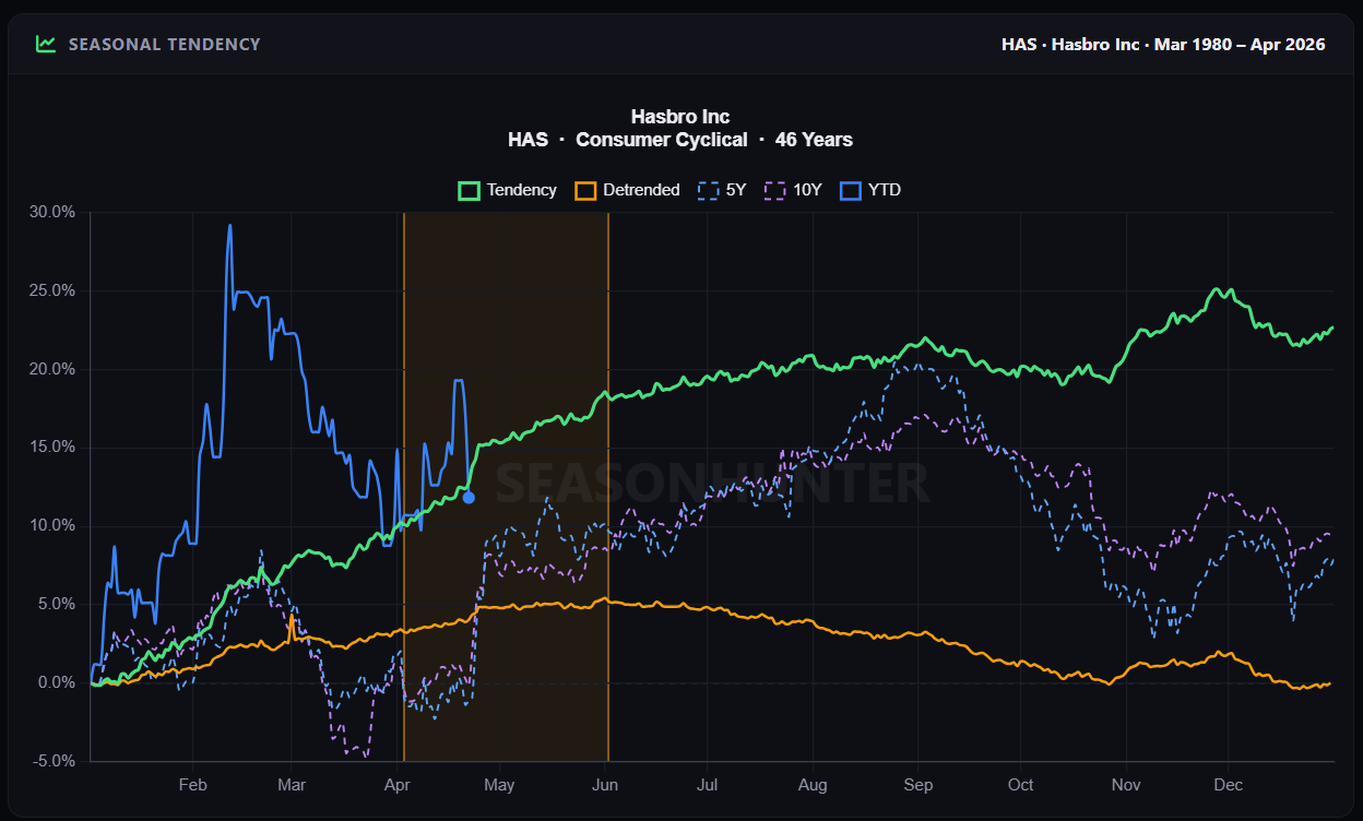
On April 1st, I ran my seasonal screening using SeasonHunter. HAS has come up with a strong recurring pattern; historically, the stock tends to drift upward during this specific window. The signal was clean: directional bias, defined seasonality, and clear entry timing.
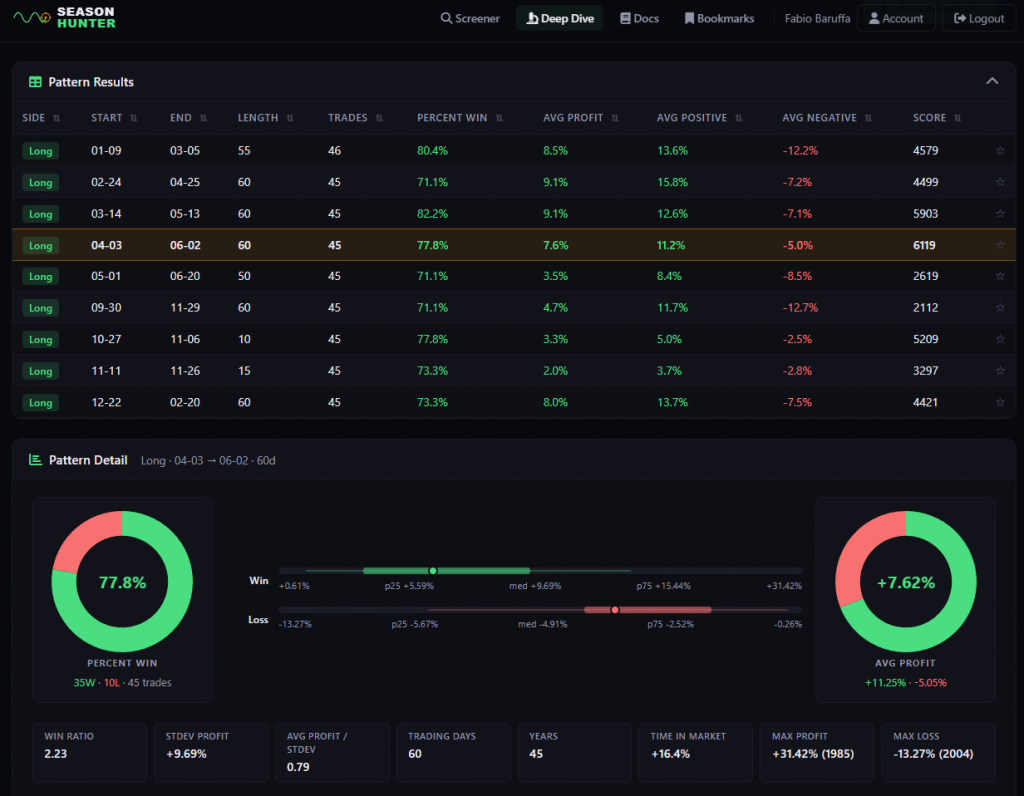
The Pattern Scanner has evaluated dozens of window combinations for HAS and ranked them by score. The highlighted row, the one I traded, is the Long 04-03 → 06-02, 60-day window, with a score of 6119. That’s the highest score on the entire list. The scanner is telling you: this is the strongest recurring seasonal window for this instrument.
Now let’s unpack the statistics.
77.8% win rate. 35 wins, 10 losses, across 45 years of data.
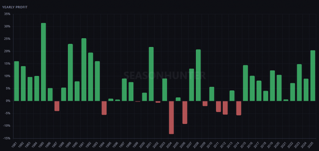
That’s not a small sample. 45 historical occurrences are enough to be statistically meaningful. Three out of every four times this trade was opened, it closed profitably. The one losing year in four is the noise you accept in exchange for the edge.
Average profit: +7.62%
But averages can lie. What matters is the distribution. Look at the percentile breakdown:
| Metric | Value |
|---|---|
| Win p25 | +5.59% |
| Win median | +9.69% |
| Win p75 | +15.44% |
| Loss median | -4.91% |
| Loss p75 (worst 25%) | -2.52% |
| Max historical profit | +31.42% (1985) |
| Max historical loss | -13.27% (2004) |
The asymmetry here is what you want to see. The median win (+9.69%) is roughly double the median loss (-4.91%). Even the weakest quartile of wins (+5.59%) outperforms the typical loss. This is the shape of a genuine edge, not a lucky streak.
Win ratio: 2.23
This means winning trades are on average 2.23x larger than losing trades. Combined with a 77.8% win rate, the expected value per trade is strongly positive. You don’t need to be right every time. You just need to be right most of the time and let the math work.
Avg Profit / StDev: 0.79
Think of this as a Sharpe-like metric for the seasonal pattern. A value above 0.5 is already solid. At 0.79, this pattern has a strong signal-to-noise ratio — the average return is large relative to the year-to-year variability. The edge is consistent, not driven by a handful of outlier years.
Time in market: 16.4%
This is one of my favourite numbers on the entire dashboard. This pattern only requires you to be exposed to market risk for 16.4% of the calendar year. You’re not sitting in the trade grinding through 12 months of noise. You’re in for a defined 60-day window with a structural tailwind, and out. The rest of the year, that capital is free for other setups.
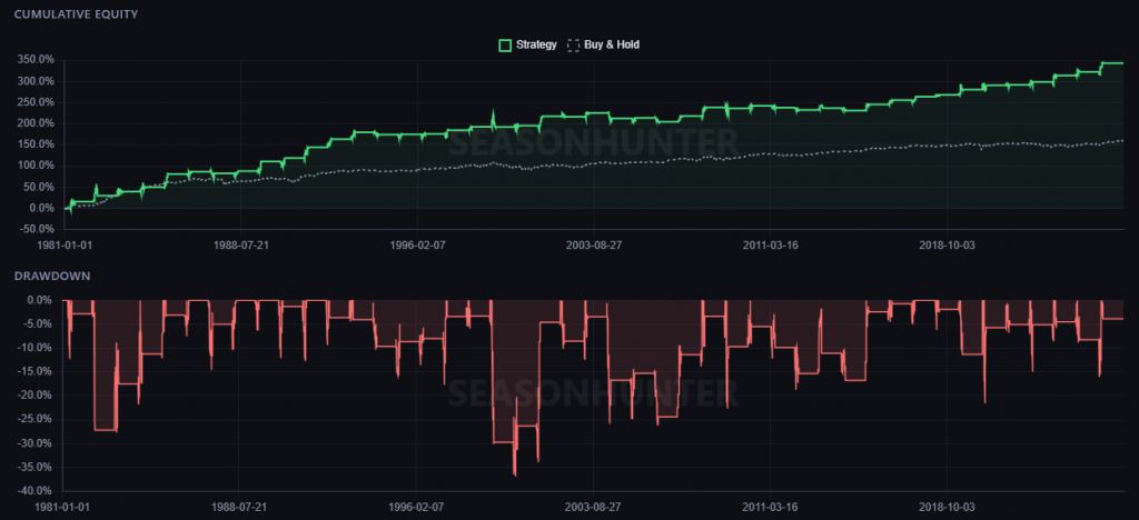
Indeed, if I had traded this seasonal pattern over all the years, I would have gained a great cumulative profit.
One more thing worth noting: look at the other rows in the scanner. The March 14 → May 13 window scores 5903 with an 82.2% win rate. The January 9 → March 5 window has an 80.4% win rate. HAS isn’t a one-trick pony; it has recurring seasonal structure across multiple windows throughout the year. That’s the kind of instrument you want in a systematic seasonal portfolio.
Trading the Signal
The April 3 window was the one opening imminently. The data was clean. I opened the trade.
Stock price at the time: ~$89.
The setup I chose was a Bull Put Spread:
| Parameter | Value |
|---|---|
| Strategy | Bull Put Spread |
| Short Put Strike | $87.50 |
| Long Put Strike | $77.50 |
| Expiration | June 18 |
| Premium Collected | $302 |
| Margin Required | ~$500 |
| Stock Price at Open | ~$89 |
The structure is simple: I sold the $87.50 put and bought the $77.50 put as protection. Maximum profit is the $302 premium if HAS stays above $87.50 at expiration. Maximum loss is capped at $698 (the $10 spread width minus the $3.02 premium collected).
The key here is the margin required: less than $500.
That number matters. I’ll come back to it.
One Week Later: The Edge Shows Up
By April 8th, roughly one week after opening the trade, HAS had moved from ~$89 to ~$93.80. A +5.3% move in the underlying.
The vertical spread, which I had sold for $302, had deflated to $214 in value.
That’s an $88 gain, or roughly 30% of the maximum profit, in about 7 trading days.
Now, some of you are reading that and thinking: $88? That’s it?
Fair. In absolute terms, it’s not a life-changing number. But here’s where it gets interesting, and why options have an intrinsic advantage over pure equity for this kind of play.
The Options Advantage: Return on Capital
Let’s do the comparison properly.
With $500 of capital in a stock trade, on April 1st, I could buy approximately 5–6 shares of HAS at $89.
Let’s say I stretch to 6 shares:
Capital deployed: 6 × $89 = $534
Value after move: 6 × $93.80 = $562.80
Profit: $28.80
Return on capital: ~5.4%
Now look at the options trade:
Margin required: ~$500
Profit captured (at +30% of max): $88
Return on capital: ~17.6%
Same capital. Same directional bet. Same underlying move.
Options: +17.6%. Equity: +5.4%.
That’s a 3x leverage factor on deployed capital, without taking on unlimited risk. The spread structure gives you a hard floor on losses. The equity position doesn’t.
This is what I mean when I say options give you intrinsic leverage with controlled risk. You’re not betting the house. You’re using capital efficiently.
April 17th: The Exit Decision
Here’s where execution matters more than theory.
By April 17th — 17 days after opening the trade — HAS was still elevated. The vertical spread had continued to deflate and was now trading at $1.40.
Let me put that in context:
| Value | |
|---|---|
| Premium collected at open | $302 |
| Spread value on April 17 | $140 |
| Profit locked in if closed | $162 |
| Days elapsed | 17 |
| Days to expiration | ~60 remaining |
The position had eroded roughly 54% of the maximum premium in just 17 days — less than a quarter of the way through the life of the trade.
I closed it.
I have a rule for premium-selling structures, and it’s simple:
If I’ve eroded more than 50% of the collected premium in less than 50% of the trade’s time horizon, I close.
In this case:
- Time elapsed: 17 days out of ~78 total = 22% of the trade’s duration
- Premium eroded: ~54% of maximum
I hit the threshold early. The trade had done its job.
The question at that point isn’t “how much more can I make?” It’s “Why am I still holding risk?”
Sixty more days of exposure, through earnings, macro events, and volatility spikes, for a potential additional $140. That math doesn’t appeal to me. I had the edge, I captured it, I moved on.
This is what systematic trading looks like: not greedy, not emotional, just disciplined.
Let me summarise the complete lifecycle:
| Date | Event | P&L |
|---|---|---|
| April 1 | Open Bull Put Spread 87.5/77.5 June | +$302 collected |
| April 8 | Spread at $214 (~30% profit) | +$88 unrealized |
| April 17 | Close position, spread at $140 | +$162 realized |
Final return on deployed capital: ~32.4% on less than $500 in 17 days.
Not life-changing. But scalable. And repeatable, because the entry was based on a statistical edge, not a gut feeling.
The Real Takeaway
A lot of traders look at seasonal patterns and think: buy the stock, ride the trend, sell at the top.
That works. But options give you a different set of tools:
Defined risk. The spread caps your loss. No stop-loss drama, no gap-down panic. You know the worst case at entry.
Capital efficiency. You’re deploying $500, not $5,000. That frees capital for other seasonal patterns, other strategies, other instruments.
Time decay as an ally. You don’t need HAS to skyrocket. You just need it to stay above $87.50. Time erodes the spread’s value whether the stock moves or stands still.
Intrinsic leverage. Same underlying move (+5.3%) delivered 3x the return on capital compared to buying shares outright.
Is position sizing still important? Absolutely. One trade at a $500 margin isn’t going to change your year. But imagine you’ve done this screening work across 20 instruments, identified 8–10 high-quality seasonal setups, and deployed capital systematically across all of them. Now the math starts to compound.
That’s the architecture behind SeasonHunter. Not a single trade — a portfolio of edges.
These aren’t speculative narratives; they’re business cycle realities that have repeated for decades. The pattern works because the underlying drivers persist.
A Question for You
I want to leave you with this:
Should I have held longer? The spread was at $1.40, expiration was 60 days away. There was $140 of premium still to erode. Some traders would have held. My rule said close.
What would you have done?
Write to me and let me know, I genuinely read every message. These discussions shape the next article.
Final Thoughts
Seasonal edges don’t need to be home runs. They need to be consistent, well-sized, and executed cleanly.
HAS gave me a +5.3% underlying move, a clean spread structure, and a disciplined exit at 54% of maximum profit in 17 days. The capital returned to the pool, ready for the next setup.
That’s the game. Not excitement — repeatability.
If you haven’t explored SeasonHunter yet, start with the free 2-week trial — no credit card needed. Run the screener, filter by your preferred entry window and win rate threshold, and see what the data surfaces. The HAS pattern I traded here is exactly the kind of setup it produces every single month across thousands of instruments.
The edge is in the data. Execution is up to you.
→ Start your free trial at SeasonHunter
This is the mindset behind The Quantitative Edge — simple ideas, implemented cleanly, that scale into powerful tools for data-driven trading.
Statemi bene!