Description
When two stocks move together over time — think Pepsi (PEP) and Coca-Cola (KO) — their price relationship often exhibits mean-reverting behavior. When one temporarily outperforms the other, the spread between them tends to snap back to its historical average. This is the foundation of pairs trading, a market-neutral strategy that profits from relative mispricings rather than directional market moves.
In this post, we’ll use Python to construct a spread between PEP and KO, calculate its z-score to identify when the spread deviates significantly from its mean, and generate trading signals based on statistical thresholds. This approach treats the spread as a stationary time series — a key assumption that we must consider and eventually test before deploying the strategy.
The z-score is a simple but powerful tool: it tells us how many standard deviations the current spread is from its historical average. When the z-score is extreme (say, +2 or -2), we have a statistical basis to expect mean reversion.
Let’s walk through the complete workflow: data collection, spread construction, z-score calculation, and signal generation.
Why Pairs Trading Works
Pairs trading exploits the principle of relative value. Like in physics, we sometimes do not care only about absolute values — we care about deviations from a reference state. Temperature anomalies, voltage fluctuations, and particle displacement are all analyzed relative to a mean and scaled by variance.
If, for example, both PEP and KO rise or fall with the broader market, their relationship often remains stable. When this relationship breaks temporarily — perhaps due to company-specific news or short-term sentiment — it creates a trading opportunity.
The strategy is quite simple:
- Go long the underperforming stock
- Go short the outperforming stock
- Wait for the spread to revert
Because you’re long one and short the other, you’re market-neutral. Your profit comes from convergence, not market direction. However, the difficulty here is to identify the relative regime between the two assets, which often depends on the time length we look for in the past.
Defining the Spread
The first step is to define a spread that captures the relative relationship between the two stocks. The simplest spread is just the difference between the two prices. However, because PEP and KO trade at different price levels, we normalize the spread using a hedge ratio.
The hedge ratio is calculated via linear regression: we regress PEP on KO to find the coefficient that minimizes the variance of the spread.
import yfinance as yf
import pandas as pd
from scipy import stats
from statsmodels.tsa.stattools import adfuller

pep = yf.Ticker("PEP")
ko = yf.Ticker("KO")

pep_data = pep.history(period='5y', interval='1d', auto_adjust=False)
ko_data = ko.history(period='5y', interval='1d', auto_adjust=False)

# Extract adjusted close prices
pep_price = pep_data['Adj Close']
ko_price = ko_data['Adj Close']

# Align the data by date
prices = pd.DataFrame({'PEP': v_price, 'KO': ma_price}).dropna()

# Calculate hedge ratio using linear regression
slope, intercept, r_value, p_value, std_err = stats.linregress(prices['PEP'], prices['KO'])

print(f"Hedge Ratio (beta): {slope:.4f}")
print(f"R-squared: {r_value**2:.4f}")

# Construct the spread
prices['Spread'] = prices['PEP'] - slope * prices['KO']This gives us synchronized daily prices for both stocks over the same time period. Hedge Ratio (beta): 0.5728
R-squared: 0.0890. The hedge ratio tells us how many shares of PEP we need to short for every share of KO we buy (or vice versa) to create a balanced position. An R-squared above 0.7 typically indicates strong cointegration — these stocks move together.
Calculate the Z-Score
The z-score standardizes the spread by expressing it in terms of standard deviations from its rolling mean.
Formula:
Z-Score = (Spread – Rolling Mean) / Rolling Std Dev
We’ll use a 20-day rolling window to capture short-term deviations.
window = 20
prices['Spread_Mean'] = prices['Spread'].rolling(window=window).mean()
prices['Spread_Std'] = prices['Spread'].rolling(window=window).std()

# Calculate z-score
prices['Z_Score'] = (prices['Spread'] - prices['Spread_Mean']) / prices['Spread_Std']

import matplotlib.pyplot as plt
plt.figure(figsize=(13,6))
plt.plot(prices.index, prices["Z_Score"], label="Z-Score")
plt.axhline(2, color="green", linestyle="--", label="+2 Threshold")
plt.axhline(0, color="gray", linestyle=":")
plt.axhline(-2, color="red", linestyle="--", label="-2 Threshold")
plt.title("Z-Score Spread (20-day)")
plt.legend()
plt.show()
A z-score of +2 means the spread is 2 standard deviations above its mean — PEP is expensive relative to KO. A z-score of -2 means the opposite — PEP is cheap relative to KO.
Generate Trading Signals
We’ll use simple threshold-based rules:
- Short the spread (short PEP, long KO) when z-score > +2
- Long the spread (long PEP, short KO) when z-score < -2
- Exit positions when z-score crosses back to 0
prices['Signal'] = 0

# Generate signals
prices.loc[prices['Z_Score'] > 2, 'Signal'] = -1  # Short spread
prices.loc[prices['Z_Score'] < -2, 'Signal'] = 1   # Long spread

# Exit when z-score crosses zero
prices['Position'] = prices['Signal'].fillna(method='ffill').fillna(0)

# Mark exits
for i in range(1, len(prices)):
    if prices['Position'].iloc[i-1] != 0:
        if (prices['Z_Score'].iloc[i-1] > 0 and prices['Z_Score'].iloc[i] < 0) or \
           (prices['Z_Score'].iloc[i-1] < 0 and prices['Z_Score'].iloc[i] > 0):
            prices['Position'].iloc[i] = 0

# Plotting
fig, (ax1, ax2) = plt.subplots(2, 1, figsize=(12, 8), sharex=True)

# Plot spread
ax1.plot(prices.index, prices['Spread'], label='Spread (PEP - β*KO)', color='blue')
ax1.axhline(prices['Spread'].mean(), color='black', linestyle='--', label='Mean')
ax1.set_ylabel('Spread ($)')
ax1.set_title('Spread Over Time')
ax1.legend()
ax1.grid(True, alpha=0.3)

# Plot z-score with signal thresholds
ax2.plot(prices.index, prices['Z_Score'], label='Z-Score', color='purple')
ax2.axhline(2, color='red', linestyle='--', label='Threshold (+2)')
ax2.axhline(-2, color='green', linestyle='--', label='Threshold (-2)')
ax2.axhline(0, color='black', linestyle='-', alpha=0.3)

# Highlight trades
long_signals = prices[prices['Signal'] == 1]
short_signals = prices[prices['Signal'] == -1]
ax2.scatter(long_signals.index, long_signals['Z_Score'], color='green', marker='^', s=100, label='Long Spread', zorder=5)
ax2.scatter(short_signals.index, short_signals['Z_Score'], color='red', marker='v', s=100, label='Short Spread', zorder=5)

ax2.set_ylabel('Z-Score')
ax2.set_xlabel('Date')
ax2.set_title('Z-Score and Trading Signals')
ax2.legend()
ax2.grid(True, alpha=0.3)

plt.tight_layout()
plt.show()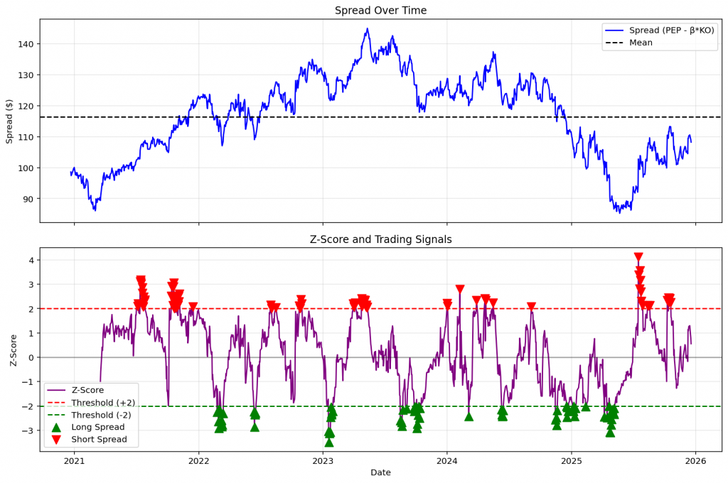
This gives you a clear visual of when extreme deviations occur and where the strategy would have triggered trades.
Backtest the Strategy
To evaluate performance, we calculate the P&L from holding the spread position.
# Calculate spread returns
prices['Spread_Return'] = prices['Spread'].pct_change()

# Calculate strategy returns
prices['Strategy_Return'] = prices['Position'].shift(1) * prices['Spread_Return']

# Cumulative returns
prices['Cumulative_Strategy'] = (1 + prices['Strategy_Return']).cumprod()

# Plot cumulative returns
plt.figure(figsize=(12, 6))
plt.plot(prices.index, prices['Cumulative_Strategy'], label='Pairs Trading Strategy', color='darkblue', linewidth=2)
plt.axhline(1, color='black', linestyle='--', alpha=0.5)
plt.title('Cumulative Returns: PEP-KO Pairs Trading Strategy')
plt.xlabel('Date')
plt.ylabel('Cumulative Return')
plt.legend()
plt.grid(True, alpha=0.3)
plt.show()

# Performance metrics
total_return = (prices['Cumulative_Strategy'].iloc[-1] - 1) * 100
sharpe = prices['Strategy_Return'].mean() / prices['Strategy_Return'].std() * np.sqrt(252)
print(f"Total Return: {total_return:.2f}%")
print(f"Sharpe Ratio: {sharpe:.2f}")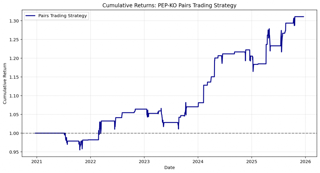
Final Thoughts
Z-score-based pairs trading is a systematic approach to capturing mean reversion between correlated stocks. By framing the spread as a statistical process and triggering trades only at extreme deviations, we create a rules-based strategy grounded in measurable probabilities.
However, several considerations matter:
- Cointegration can break — economic or structural changes can decouple previously stable relationships
- Transaction costs — frequent rebalancing can erode profits, especially with small z-score thresholds
- Parameter sensitivity — the choice of rolling window and z-score threshold significantly affects results
- Regime changes — correlations weaken during crises or sector rotations
Before deploying capital, test multiple pairs, vary the window lengths, and stress-test under different market conditions. The z-score is a starting point, not a guarantee.
This is the mindset behind The Quantitative Edge — rigorous testing, clean implementation, and evidence-based decisions that turn statistical patterns into tradable strategies.
Statemi bene!