Description
In the previous post on Spread Trading with Z-Score, I walked through a complete pairs trading workflow using PEP and KO: constructing the spread, calculating the z-score, generating signals, and running a basic backtest. It was a clean, working implementation designed to demonstrate the method clearly.
But I was deliberate about something. That first version used a static hedge ratio; one slope calculated over the full 5-year history. I kept it that way intentionally to focus on the concept without layering in too much complexity at once.
Now it’s time to fix it. Because in production, that static slope is a ticking time bomb.
The Problem: Relationships Don’t Stay Still
Think of it this way. You run a linear regression on 5 years of PEP and KO data and get a hedge ratio of, say, 0.57. That number becomes the backbone of your entire strategy. Every signal, every trade, every z-score: all derived from that single coefficient.
Here’s the question you should be asking: Was that relationship stable for all 5 years?
Almost certainly not. The two stocks live in the same sector, but they’re not the same company. Earnings cycles, management changes, dividend adjustments, and macro regimes: all of these create drift in the relative pricing. What was a stable relationship in 2020 may look completely different in 2024.
When you use a static slope, you’re doing two dangerous things:
- Introducing look-ahead bias. The slope is calculated using data you wouldn’t have had at the time of each trade.
- Hiding regime changes inside the spread. If the relationship between PEP and KO drifts over time, the “spread” you’re measuring is partly capturing that drift, not genuine mean reversion opportunities.
The z-score assumes the spread is stationary. A static slope applied to a non-stationary relationship violates that assumption silently.
The Fix: Rolling OLS Regression
The solution is to recalculate the hedge ratio at every point in time using only a lookback window of past data. This is called a rolling OLS (Ordinary Least Squares) regression.
The idea is simple: at each day t, we fit a linear regression using the previous N days, extract the slope, and use that slope to construct the spread for that day t. The slope becomes a time series rather than a single number.
import yfinance as yf
import pandas as pd
import numpy as np
import matplotlib.pyplot as plt

# Download data
pep_data = yf.Ticker("PEP").history(period='5y', interval='1d', auto_adjust=False)
ko_data  = yf.Ticker("KO").history(period='5y', interval='1d', auto_adjust=False)

pep_price = pep_data['Adj Close']
ko_price  = ko_data['Adj Close']

prices = pd.DataFrame({'PEP': pep_price, 'KO': ko_price}).dropna()Now the rolling slope calculation, assuming a lookback period of 60 days :
window = 60  # 60-day lookback for the hedge ratio

rolling_slope = []

for i in range(len(prices)):
    if i < window:
        rolling_slope.append(np.nan)
    else:
        y = prices['PEP'].iloc[i - window:i].values
        x = prices['KO'].iloc[i - window:i].values
        # np.polyfit returns [slope, intercept]
        slope, _ = np.polyfit(x, y, 1)
        rolling_slope.append(slope)

prices['Rolling_Slope'] = rolling_slopeThis is clean and explicit. It is just a rolling window of linear regression at each step. The first 60 rows will be NaN because we don’t have enough history yet. That’s correct and expected from a rolling calculation.
Now construct the spread using the time-varying slope:
prices['Spread'] = prices['PEP'] - prices['Rolling_Slope'] * prices['KO']Visualizing the Slope Drift
Before doing anything else with the spread, plot the rolling slope. This is the most important diagnostic step.
plt.figure(figsize=(13, 4))
plt.plot(prices.index, prices['Rolling_Slope'], color='steelblue', linewidth=1.5)
plt.axhline(prices['Rolling_Slope'].mean(), color='black', linestyle='--', alpha=0.5, label='Mean slope')
plt.title('Rolling 60-Day Hedge Ratio: PEP vs KO')
plt.ylabel('Slope (β)')
plt.legend()
plt.grid(True, alpha=0.3)
plt.tight_layout()
plt.show()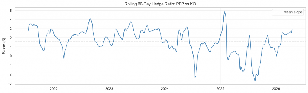
If the slope is relatively flat over time, the static approach wasn’t catastrophically wrong. If it swings significantly, like in mostly pairs, it is proof that the static hedge ratio was silently absorbing structural drift into your spread signal.
Recalculate the Z-Score
With the dynamic spread constructed, the z-score calculation is identical to the previous post. The only difference is that the spread now accurately reflects the current relationship between the two stocks. We also plot the z-score to see how it compares to the version from the previous post. We use the same rolling window of 20 days, like in the previous post.
z_window = 20  # rolling window for z-score normalization

prices['Spread_Mean'] = prices['Spread'].rolling(window=z_window).mean()
prices['Spread_Std']  = prices['Spread'].rolling(window=z_window).std()
prices['Z_Score']     = (prices['Spread'] - prices['Spread_Mean']) / prices['Spread_Std']

prices_clean = prices.dropna()

plt.figure(figsize=(13, 5))
plt.plot(prices_clean.index, prices_clean['Z_Score'], color='purple', linewidth=1)
plt.axhline( 2, color='green', linestyle='--', label='+2 Threshold')
plt.axhline( 0, color='gray',  linestyle=':')
plt.axhline(-2, color='red',   linestyle='--', label='-2 Threshold')
plt.title('Z-Score with Rolling Hedge Ratio (60-day slope, 20-day z-score)')
plt.legend()
plt.grid(True, alpha=0.3)
plt.tight_layout()
plt.show()You will immediately notice a difference in the signal behavior. With a static slope, the spread can drift systematically in one direction for months, generating false signals that appear to be mean-reversion opportunities but are actually just regime drift. With the rolling slope, the spread stays anchored to the current relationship, and the z-score oscillates more cleanly around zero.
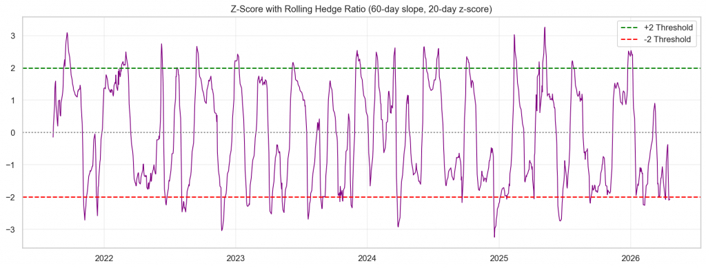
A z-score of +2 means the spread is 2 standard deviations above its mean: PEP is expensive relative to KO. A z-score of -2 means the opposite: PEP is cheap relative to KO.
Generate Trading Signals
The signal logic is unchanged from the previous post. We’ll use simple threshold-based rules:
- Short the spread (short PEP, long KO) when z-score > +2
- Long the spread (long PEP, short KO) when z-score < -2
- Exit positions when the z-score crosses back to 0
prices_clean = prices.dropna().copy()
prices_clean['Signal'] = 0

prices_clean.loc[prices_clean['Z_Score'] >  2, 'Signal'] = -1  # Short spread
prices_clean.loc[prices_clean['Z_Score'] < -2, 'Signal'] =  1  # Long spread

# Forward-fill position, then exit on zero crossing
prices_clean['Position'] = prices_clean['Signal'].replace(0, np.nan).ffill().fillna(0)

# Exit when z-score crosses zero
position = prices_clean['Position'].values
z = prices_clean['Z_Score'].values

for i in range(1, len(position)):
    if position[i-1] != 0:
        if (z[i-1] > 0 and z[i] < 0) or (z[i-1] < 0 and z[i] > 0):
            position[i] = 0

prices_clean['Position'] = positionThe Backtest
With the dynamic spread and z-score in place, the signal logic is the same as in the previous post, but now it operates on a spread that reflects the current relationship between the two stocks. Short when the z-score is too high, long when it is too low, and exit when it crosses back to zero.
The profit and loss of the strategy is measured in dollar terms: the cumulative sum of daily spread changes captured while in position. This is the natural unit for a spread strategy. Unlike a single stock, where percentage returns make intuitive sense, a spread is a price difference. It has no meaningful “base” to normalize against. What matters is how many dollars the spread moved in your favor while you were holding the position. That is what the equity curve shows.
# Spread_Change: dollar change, not percentage
prices_clean['Spread_Change']       = prices_clean['Spread'].diff()
prices_clean['Strategy_Return']     = -prices_clean['Position'].shift(1) * prices_clean['Spread_Change']
prices_clean['Cumulative_Strategy'] = prices_clean['Strategy_Return'].cumsum()

total_pnl = prices_clean['Cumulative_Strategy'].iloc[-1]
sharpe    = prices_clean['Strategy_Return'].mean() / prices_clean['Strategy_Return'].std() * np.sqrt(252)
max_dd    = (prices_clean['Cumulative_Strategy'] - prices_clean['Cumulative_Strategy'].cummax()).min()

print(f"% time in market : {(prices_clean['Position'] != 0).mean():.1%}")
print("── Performance Metrics ───────────────────")
print(f"Total P&L        : ${total_pnl:.2f}")
print(f"Sharpe Ratio     : {sharpe:.2f}")
print(f"Max Drawdown     : ${max_dd:.2f}")
print("──────────────────────────────────────────")──────────────────────────────────────────
% time in market : 60.1%
── Performance Metrics ───────────────────
Total P&L : $1329.85
Sharpe Ratio : 3.00
Max Drawdown : $-119.67
──────────────────────────────────────────
Total trades : 34
Long entries : 18 (long PEP / short KO)
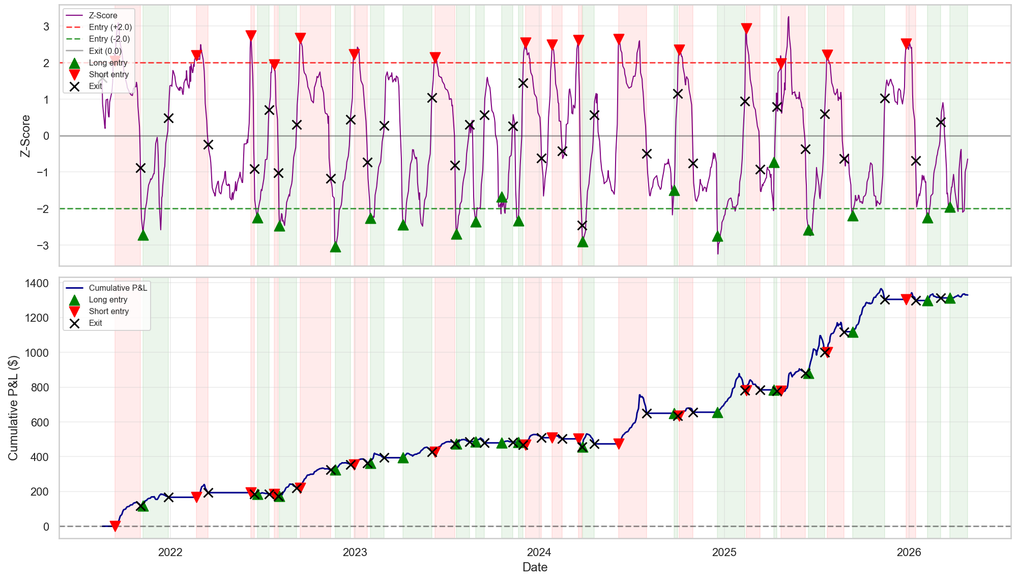
Short entries : 16 (short PEP / long KO)The backtest on PEP/KO delivers a total P&L of $1,329 across 34 trades with a Sharpe ratio of 3.00 and a maximum drawdown of only $119. The strategy spent 60% of the time in the market, splitting entries evenly between long and short spread positions, suggesting the z-score signals are firing symmetrically around the mean rather than being biased in one direction.
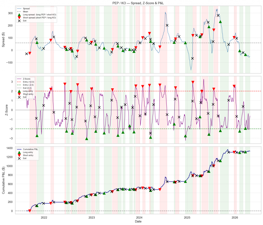
The top panel shows the spread oscillating around its mean. The central panel shows the z-score with entry signals marked: green triangles for long entries, red triangles for short entries. With the rolling hedge ratio, the spread is far more stationary than its static counterpart. The signals are anchored to a relationship that is measured in real time, not averaged across five years of history. The bottom panel is the cumulative return of the spread.
Known Limitations
This framework is built on solid statistical foundations, but it comes with limitations that every honest systematic trader should understand before deploying real capital.
Two Parameters, Two Decisions
There is one thing that deserves explicit attention: you now have two separate window parameters.
- window = 60: the lookback for the hedge ratio (slope)
- z_window = 20: the lookback for the z-score normalization
These are independent decisions, and they control different things.
The slope window controls how quickly the hedge ratio adapts to structural changes in the relationship. A shorter window makes it more responsive but also noisier. A longer window is more stable but slower to detect regime shifts. 60 days is a reasonable starting point for daily data.
The z-score window controls how sensitive your signal is to short-term deviations. This hasn’t changed from the original post; 20 days captures short-term oscillations effectively.
Both parameters need to be tested. There is no universal answer. Use your own walk-forward analysis to find what works for the specific pair you’re trading.
Cointegration
Ignoring the cointegration. Cointegration is a statistical property that describes a stable long-term relationship between two non-stationary price series. Individual stock prices are like random walks; they drift without a fixed mean, making them inherently unpredictable in level terms. But two stocks can be individually unpredictable while their combination – the spread – behaves like a stationary process that oscillates around a stable mean. That is cointegration. Think of it as two drunk people walking home separately: each follows an erratic, unpredictable path. But if they are connected by a leash, the distance between them stays bounded. The leash is the cointegrating relationship. In pairs trading, cointegration is what transforms a speculative directional bet into a mean-reversion strategy grounded in statistical theory. Without it, the spread you are trading has no anchor; it can drift indefinitely in one direction, and every signal you generate is built on a foundation that does not exist. With it, deviations from the mean are temporary by definition, and the z-score becomes a meaningful measure of how far the relationship has stretched and how likely it is to snap back. This is why testing for cointegration is not a preliminary step you run once and forget. This is the central question that the entire strategy depends on.
Final Thoughts
The previous post was designed to be a clear, accessible introduction to z-score-based pairs trading. The static slope served that purpose well: it kept the focus on the mechanics without adding unnecessary complexity.
But simplified versions are starting points, not finished strategies.
The rolling hedge ratio is not an optional refinement. It is the correct way to construct a pairs trading spread when you expect the relationship between two assets to evolve over time. Without it, you are trading a signal that is partly driven by a structural drift you never intended to measure.
Two things to take away:
The window length matters. Experiment with different lookbacks, both for the slope and the z-score. There is no right answer, only empirically supported answers for your specific pair and time period.
Stationarity is not given; it must be earned. Before constructing the rolling spread over a pair, always test the cointegration with an Augmented Dickey-Fuller test. This can give you an indication of the signal it generates. If the spread isn’t stationary, the z-score is not what you think it is.
This is what systematic trading looks like: start with the concept, implement the simplified version to understand the mechanics, then replace every assumption with something you can measure and defend.
This is the mindset behind The Quantitative Edge — rigorous testing, clean implementation, and evidence-based decisions that turn statistical patterns into tradable strategies.
Statemi bene!
If you found this useful, you might also enjoy: